Accessing CEFI data with Python#
Packages used#
To use python to access the ERDDAP server directly from your python script or jupyter-notebook, you will need
Xarray
netcdf4
matplotlib
folium
Packages
The package netcdf4 develop by UNIDATA is not needed in the import part of the python script. However, it is the essential package that support netCDF format output from Xarray and OPeNDAP access. The package matplotlib is also not needed in the import part of the python script. It is the essential package that support quick visualization from Xarray.
On this page, we will explore the process of extracting a subset of model simualtion data produce from the regional MOM6 model. The model output is to support the Changing Ecosystem and Fishery Initiative. We will showcase how to utilize OPeNDAP for accessing the data and visualize it on an interactive map. The currently available data can be viewed here. The contents of this folder encompass historical simulations derived from the regional MOM6 model spanning the years 1993 to 2019.
Import python packages#
import xarray as xr
Info
Thanks to the netCDF4/Pydap library, accessing data through OPeNDAP directly from Xarray is made seamless. For detailed usage guidance, the Xarray documentation offers excellent examples and explanations. Ex: if the OPeNDAP server require authentication, backends.PydapDataStore can help on storing the login data.
Access data (regular grid product)#
From the previous page explaining OPeNDAP interface, we know that the OPeNDAP URL can be obtained from the form. In our case, we will get the URL from this form
opendap_url = "http://psl.noaa.gov/thredds/dodsC/Projects/CEFI/regional_mom6/northwest_atlantic/hist_run/regrid/ocean_monthly.199301-201912.ssh.nc"
ds_ssh = xr.open_dataset(opendap_url)
ds_ssh
<xarray.Dataset> Size: 847MB
Dimensions:  (lon: 774, lat: 844, time: 324)
Coordinates:
  * lon      (lon) float64 6kB 261.6 261.6 261.7 261.8 ... 323.8 323.8 323.9
  * lat      (lat) float64 7kB 5.273 5.335 5.398 5.461 ... 58.04 58.1 58.16
  * time     (time) datetime64[ns] 3kB 1993-01-16T12:00:00 ... 2019-12-16T12:...
Data variables:
    ssh      (time, lat, lon) float32 847MB ...
Attributes:
    NumFilesInSet:       1
    title:               NWA12_COBALT_2023_04_kpo4-coastatten-physics
    associated_files:    areacello: 19930101.ocean_static.nc
    grid_type:           regular
    grid_tile:           N/A
    external_variables:  areacello
    history:             Derived and written at NOAA Physical Science Laboratory
    NCO:                 netCDF Operators version 5.0.1 (Homepage = http://nc...
    contact:             chia-wei.hsu@noaa.gov
    dataset:             regional mom6 regrid
_NCProperties: version=2,netcdf=4.9.2,hdf5=1.14.3Tip
When we use xr.open_dataset() to load the data from OPeNDAP, we actually only load the metadata and coordinates information. This provide a great way to peek at the data’s dimension and availability on our local machine in the xarray object format. The actual gridded data values at each grid point will only be downloaded from the PSL server when we add .load() to the dataset.
Since most OPeNDAP server will set a single time data transfer limit (PSL server has a 500MB limit), we cannot ds_ssh.load() the whole dataset. However, we can load the sea level map at a single time step which is smaller than 500MB.
ds_ssh_subset = ds_ssh.sel(time='2012-12').load()
ds_ssh_subset
<xarray.Dataset> Size: 3MB
Dimensions:  (lon: 774, lat: 844, time: 1)
Coordinates:
  * lon      (lon) float64 6kB 261.6 261.6 261.7 261.8 ... 323.8 323.8 323.9
  * lat      (lat) float64 7kB 5.273 5.335 5.398 5.461 ... 58.04 58.1 58.16
  * time     (time) datetime64[ns] 8B 2012-12-16T12:00:00
Data variables:
    ssh      (time, lat, lon) float32 3MB nan nan nan nan ... nan nan nan nan
Attributes:
    NumFilesInSet:       1
    title:               NWA12_COBALT_2023_04_kpo4-coastatten-physics
    associated_files:    areacello: 19930101.ocean_static.nc
    grid_type:           regular
    grid_tile:           N/A
    external_variables:  areacello
    history:             Derived and written at NOAA Physical Science Laboratory
    NCO:                 netCDF Operators version 5.0.1 (Homepage = http://nc...
    contact:             chia-wei.hsu@noaa.gov
    dataset:             regional mom6 regrid
_NCProperties: version=2,netcdf=4.9.2,hdf5=1.14.3From the xarray dataset object output above, we will notice the ssh value in ds_ssh_subset is now avaible and printed out while the ssh value in ds_ssh is not. This means the ssh values has been downloaded from the OPeNDAP server to the local machine memory.
Read the data by chunk#
Leveraging Xarray and Dask, we can load data lazily—initially retrieving only metadata and coordinate information. This allows us to inspect the dataset’s structure and dimensions without downloading the full data. The actual variable values (such as sea surface height or O2 at each grid point) are only fetched from the PSL server when we perform further operations, like subsetting or aggregation.
How are chunks related to lazy loading?
Dask provides an excellent overview of the concept of “chunks.” Instead of loading an entire netCDF file into memory, the data is divided into smaller, manageable pieces called chunks (for example, a 20x20 grid can be split into four 10x10 chunks). Dask reads and processes these chunks only when needed, allowing computations to be performed efficiently without exceeding memory limits.
To manually enable chunking—Xarray with Dask, one can just set chunks={}, using a chunking scheme that matches the original netCDF file’s native chunking. This ensures efficient memory usage and computation without additional configuration.
With lazy-loading, only metadata and coordinate information are loaded initially. The actual data values are accessed and loaded into memory only when you perform computations or visualizations.
Using the 3D ds_o2 dataset as an example (which is well above the 1GB limit of the PSL OPeNDAP server), chunking is essential to safely load and process the data.
opendap_url = 'http://psl.noaa.gov/thredds/dodsC/Projects/CEFI/regional_mom6/cefi_portal/northwest_atlantic/full_domain/hindcast/monthly/regrid/r20250715/o2.nwa.full.hcast.monthly.regrid.r20250715.199301-202312.nc'
ds_o2 = xr.open_dataset(opendap_url,chunks={})
Quick lazy-loading allows us to easily view the dataset’s metadata and coordinates below.
ds_o2
<xarray.Dataset> Size: 51GB
Dimensions:  (time: 372, z_l: 52, lon: 774, lat: 844)
Coordinates:
  * time     (time) datetime64[ns] 3kB 1993-01-16T12:00:00 ... 2023-12-16T12:...
  * z_l      (z_l) float64 416B 2.5 7.5 12.5 17.5 ... 5.25e+03 5.75e+03 6.25e+03
  * lon      (lon) float64 6kB -98.44 -98.36 -98.28 ... -36.24 -36.16 -36.08
  * lat      (lat) float64 7kB 5.273 5.335 5.398 5.461 ... 58.04 58.1 58.16
Data variables:
    o2       (time, z_l, lat, lon) float32 51GB dask.array<chunksize=(372, 52, 844, 774), meta=np.ndarray>
Attributes: (12/28)
    NumFilesInSet:          1
    title:                  NWA12_COBALT_2025_04_bugfixes
    associated_files:       areacello: 19930101.ocean_static.nc
    grid_type:              regular
    grid_tile:              N/A
    external_variables:     volcello areacello
    ...                     ...
    cefi_ensemble_info:     N/A
    cefi_forcing:           N/A
    cefi_data_doi:          10.5281/zenodo.7893386
    cefi_paper_doi:         10.5194/gmd-16-6943-2023
    cefi_aux:               Postprocessed Data : regrid to regular grid
_NCProperties: version=2,netcdf=4.9.2,hdf5=1.14.3Tip!
When working with large netCDF files, OPeNDAP server requests can be slow to process, especially for large subsets. Always start by requesting the smallest possible subset to quickly inspect the data before attempting larger downloads. If you encounter a DAP error, it may indicate that the server is ignoring chunking due to its configuration. In such cases, manually concatenating smaller subsets is often necessary to acquire larger datasets efficiently.
Sometimes, even if the subset you request is small, you may still encounter a DAP error. This often happens because the netCDF file is internally chunked, and if your requested slice overlaps with a large chunk, the server must read and transfer the entire chunk. As a result, the data volume can easily exceed the server’s transfer limit for certain dimensions (such as depth). We recommand concat the data after loading small slices one step at a time like what is shown below to side step the restriction.
Since different users will have different data subsets in mind, it is difficult to find an “optimal” chunking scheme for every use case. Unfortunately, this is a downside of netCDF chunking when using OPeNDAP servers. If chunking causes issues or slows down your analysis, we recommend accessing the data from commercial cloud storage, such as AWS S3. See Accessing CEFI data on the cloud for more details.
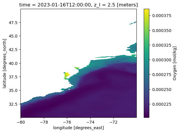
ds_o2_202301_1= ds_o2.sel(time='2023-01',lon=slice(-80,-70),lat=slice(30,40),z_l=2.5).load()
ds_o2_202301_2 = ds_o2.sel(time='2023-01',lon=slice(-80,-70),lat=slice(40,50),z_l=2.5).load()
ds_o2_202301 = xr.concat([ds_o2_202301_1, ds_o2_202301_2], dim='lat')
ds_o2_202301.o2.plot()
<matplotlib.collections.QuadMesh at 0x7f57e0b56740>
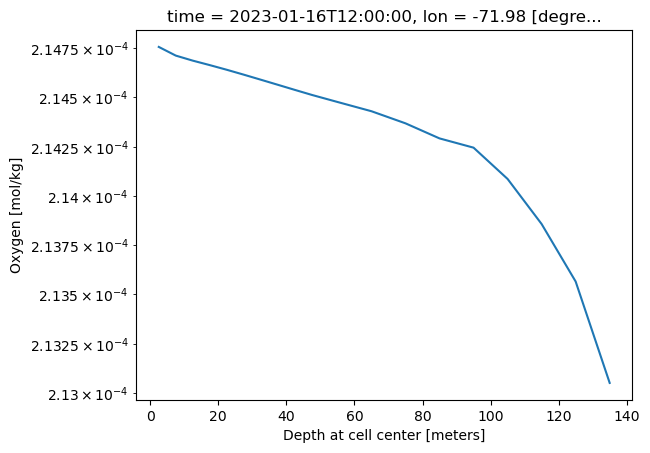
ds_o2_202301_depth1 = ds_o2.sel(time='2023-01',lon=-72,lat=32,method='nearest').sel(z_l=slice(2.5, 24.5)).load()
ds_o2_202301_depth2 = ds_o2.sel(time='2023-01',lon=-72,lat=32,method='nearest').sel(z_l=slice(24.5, 135)).load()
ds_o2_202301_depth = xr.concat([ds_o2_202301_depth1, ds_o2_202301_depth2], dim='z_l')
ds_o2_202301_depth.o2.plot(yscale='log')
[<matplotlib.lines.Line2D at 0x7f57e0ae9990>]
Quick view of the variable#
To check if the data makes sense and fits the chosen time and region, you can use Xarray’s .plot() method. This way, you see a graph instead of just numbers, making it easier to understand.
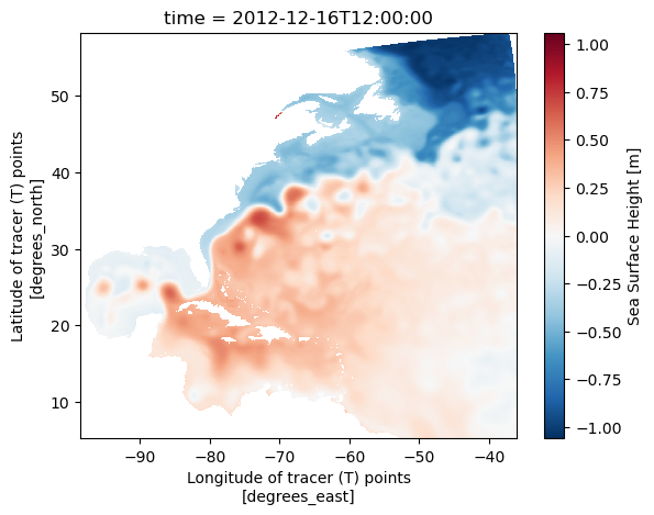
ds_ssh_subset.ssh.plot()
<matplotlib.collections.QuadMesh at 0x7f57c079f280>
Science info
The map illustrates a clear distinction between high sea levels, primarily from tropical regions (hot and fresh water), and low sea levels, mainly from the Labrador Sea or other polar areas (cold and salty sea water). The meandering pattern of the sharp sea level gradient, indicating rapid sea level changes over a short distance, highlights the location of the Gulf Stream. This distinctive sea level feature is a result of the existence of western boundary currents, commonly observed on the western edges of major ocean basins, such as the Kuroshio in the Pacific basin.
Plotting the data on a interactive leaflet map#
In this section, there are more detail figure manipulation to produce the map shown above and be able to zoom in and out from a interactive map. This is not neccessary for data downloading and preprocessing. However, this shows how the map on the CEFI portal is generated.
Load package for the interactive map#
matplotlibto generate the color shaded map abovefoliumthe python interface of generating a leaflet interactive mapbrancathe colorbar module included when installing folium package
import matplotlib.pyplot as plt
import folium
import branca.colormap as cm
Specify figure setup#
# figure setting
colormap_name = 'RdBu_r'              # colormap name in matplotlib colormap blue to red
n_increments = 20                     # number of increment in the colormap
varmin = -1                           # minimum value on the colorbar
varmax = 1                            # maximum value on the colorbar
varname = 'Sea Surface Height'        # legend show on map
da_regrid_data = ds_ssh_subset['ssh'] # Xarray DataArray object used to plot the map
Create RGBA code for each grid point#
This part use the matplotlib to create a special map (2D) which assigns a RGBA code (an array of four number) for each grid point.
This will create a array with the size of [nlon,nlat,4].
# setup the colormap from matplotlib
picked_cm = plt.get_cmap(colormap_name, n_increments)
# normalized data (0,1) for colormap to applied on
normed_data = (da_regrid_data - varmin) / (varmax - varmin)
colored_data = picked_cm(normed_data.data[0,:,:])
colored_data.shape
(844, 774, 4)
Start the base map from folium#
# folium map base map
fm = folium.Map(
    location=[float(da_regrid_data.lat.mean().data), float(da_regrid_data.lon.mean().data)],
    tiles="Cartodb Positron",
    zoom_start=3
)
Overlay the colored data on the map#
folium.raster_layers.ImageOverlay(
    image=colored_data,
    bounds=[[float(da_regrid_data.lat.min().data),
             float(da_regrid_data.lon.min().data)],
            [float(da_regrid_data.lat.max().data),
             float(da_regrid_data.lon.max().data)]],
    mercator_project=True,   # applied data to web mercator projection (essential)
    origin="lower",          # plot data from lower bound (essential)
    opacity=1,
    zindex=1
).add_to(fm)
<folium.raster_layers.ImageOverlay at 0x7f57c06383d0>
Create the colorbar for the interactive map#
import numpy as np
tick_inc = np.abs(varmax-varmin)/10.

# start constructing the branca colormap to put on folium map
index_list = range(0,n_increments)
cmap_list = picked_cm(range(n_increments)).tolist()
cmap_foliump = cm.LinearColormap(
    colors=cmap_list,
    vmin=varmin,
    vmax=varmax,
    caption='fcmap',
    max_labels=n_increments+1,
    tick_labels=list(np.arange(varmin,varmax+tick_inc*0.000001,tick_inc))
).to_step(n_increments)

# Add the colormap to the folium map
cmap_foliump.caption = varname
cmap_foliump.add_to(fm)
fm
Access data (raw grid product)#
The raw grid product differs from the regular grid in that it represents the original output of the model. The model grid uses the Arakawa C grid. The MOM6 documentation provides an excellent visualization of the Arakawa C grid. We can concentrate on the h point, which is where scalar values like sea level height are stored. The grid does not have uniform spacing and is, in fact, a curvilinear grid.
Info
The raw model output is beneficial when calculating the energy budget, which includes factors like heat and momentum. This output preserves each term’s original values, avoiding any potential distortions caused by interpolation. By using the raw grid product, we can ensure the energy budget balances within a closed system.
To use the raw grid data, one need to get two files.
the variable file
the static file
opendap_url = "http://psl.noaa.gov/thredds/dodsC/Projects/CEFI/regional_mom6/northwest_atlantic/hist_run/ocean_monthly.199301-201912.ssh.nc"
ds_ssh = xr.open_dataset(opendap_url)

opendap_static_url = "http://psl.noaa.gov/thredds/dodsC/Projects/CEFI/regional_mom6/northwest_atlantic/hist_run/ocean_static.nc"
ds_static = xr.open_dataset(opendap_static_url)
ds_ssh
<xarray.Dataset> Size: 849MB
Dimensions:     (time: 324, nv: 2, xh: 775, yh: 845)
Coordinates:
  * nv          (nv) float64 16B 1.0 2.0
  * time        (time) datetime64[ns] 3kB 1993-01-16T12:00:00 ... 2019-12-16T...
  * xh          (xh) float64 6kB -98.0 -97.92 -97.84 ... -36.24 -36.16 -36.08
  * yh          (yh) float64 7kB 5.273 5.352 5.432 5.511 ... 51.9 51.91 51.93
Data variables:
    average_DT  (time) timedelta64[ns] 3kB ...
    average_T1  (time) datetime64[ns] 3kB ...
    average_T2  (time) datetime64[ns] 3kB ...
    ssh         (time, yh, xh) float32 849MB ...
    time_bnds   (time, nv) datetime64[ns] 5kB ...
Attributes:
    NumFilesInSet:                   1
    title:                           NWA12_COBALT_2023_04_kpo4-coastatten-phy...
    associated_files:                areacello: 19930101.ocean_static.nc
    grid_type:                       regular
    grid_tile:                       N/A
    external_variables:              areacello
    history:                         Fri May 12 10:49:27 2023: ncks -4 -L 3 o...
    NCO:                             netCDF Operators version 5.0.1 (Homepage...
    _NCProperties:                   version=2,netcdf=4.9.0,hdf5=1.12.2
DODS_EXTRA.Unlimited_Dimension: timeds_static
<xarray.Dataset> Size: 66MB
Dimensions:       (time: 1, xh: 775, xq: 776, yh: 845, yq: 846)
Coordinates:
  * time          (time) datetime64[ns] 8B 1980-01-01
  * xh            (xh) float64 6kB -98.0 -97.92 -97.84 ... -36.24 -36.16 -36.08
  * xq            (xq) float64 6kB -98.04 -97.96 -97.88 ... -36.2 -36.12 -36.04
  * yh            (yh) float64 7kB 5.273 5.352 5.432 5.511 ... 51.9 51.91 51.93
  * yq            (yq) float64 7kB 5.233 5.312 5.392 5.472 ... 51.9 51.92 51.94
Data variables: (12/25)
    Coriolis      (yq, xq) float32 3MB ...
    areacello     (yh, xh) float32 3MB ...
    areacello_bu  (yq, xq) float32 3MB ...
    areacello_cu  (yh, xq) float32 3MB ...
    areacello_cv  (yq, xh) float32 3MB ...
    deptho        (yh, xh) float32 3MB ...
    ...            ...
    geolon_v      (yq, xh) float32 3MB ...
    sftof         (yh, xh) float32 3MB ...
    wet           (yh, xh) float32 3MB ...
    wet_c         (yq, xq) float32 3MB ...
    wet_u         (yh, xq) float32 3MB ...
    wet_v         (yq, xh) float32 3MB ...
Attributes:
    _NCProperties:                   version=2,netcdf=4.9.0,hdf5=1.12.2
    NumFilesInSet:                   1
    title:                           NWA12_MOM6_v1.0
    grid_type:                       regular
    grid_tile:                       N/A
    history:                         Fri May 12 10:50:21 2023: ncks -4 -L 3 o...
    NCO:                             netCDF Operators version 5.0.1 (Homepage...
DODS_EXTRA.Unlimited_Dimension: timeTip
Again, only the metadata and coordinate information are loaded into local memory, not the actual data. The gridded data values at each grid point are only downloaded from the PSL server when we append .load() to the dataset.
Warning
In the ds_static dataset, you can observe the one-dimensional xh, yh grid. The numbers on this grid may resemble longitude and latitude values, but they do not represent actual geographical locations. For accurate longitude and latitude data, you should refer to the geolon, geolat variables in the list. These variables, which are dimensioned by xh, yh, provide the correct geographical coordinates.
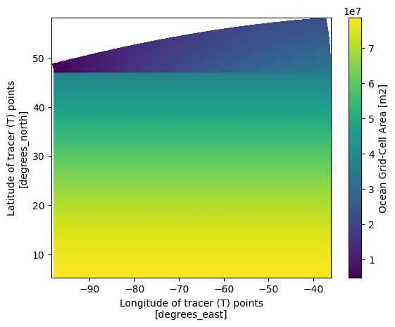
Now let’s take a look at the grid area distribution which give a great sense of how it is different from regular spacing grid
ds_static = ds_static.set_coords(['geolon','geolat'])
ds_static.areacello.plot(x='geolon',y='geolat')
<matplotlib.collections.QuadMesh at 0x7f57bbedc460>
ds_static.areacello.plot(x='xh',y='yh')
<matplotlib.collections.QuadMesh at 0x7f57bbdd4370>
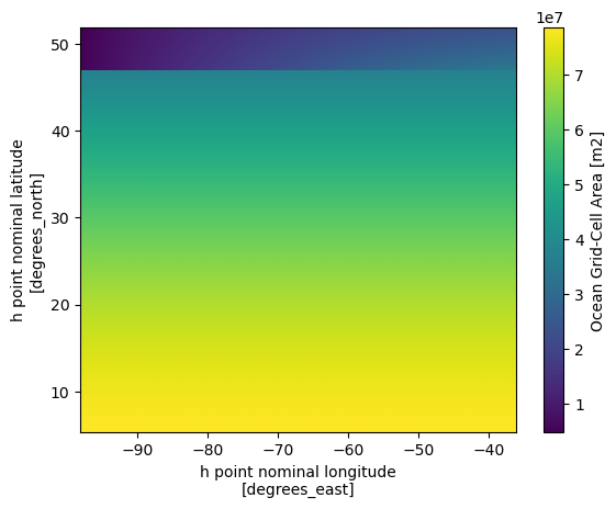
We can see that the most significant differences between the two maps are located in the higher latitudes. Since the grid information is important in the raw grid, the easiest way to merge the two dataset so we can have the accurate lon lat that follows the data that we are going to work on.
ds_ssh_subset = ds_ssh.sel(time='2012-12').load()
ds = xr.merge([ds_ssh_subset,ds_static])
ds = ds.isel(time=slice(1,None))  # exclude the 1980 empty field due to merge
ds
<xarray.Dataset> Size: 68MB
Dimensions:       (nv: 2, time: 1, xh: 775, yh: 845, xq: 776, yq: 846)
Coordinates:
  * nv            (nv) float64 16B 1.0 2.0
  * time          (time) datetime64[ns] 8B 2012-12-16T12:00:00
  * xh            (xh) float64 6kB -98.0 -97.92 -97.84 ... -36.24 -36.16 -36.08
  * yh            (yh) float64 7kB 5.273 5.352 5.432 5.511 ... 51.9 51.91 51.93
  * xq            (xq) float64 6kB -98.04 -97.96 -97.88 ... -36.2 -36.12 -36.04
  * yq            (yq) float64 7kB 5.233 5.312 5.392 5.472 ... 51.9 51.92 51.94
    geolat        (yh, xh) float32 3MB ...
    geolon        (yh, xh) float32 3MB ...
Data variables: (12/28)
    average_DT    (time) timedelta64[ns] 8B 31 days
    average_T1    (time) datetime64[ns] 8B 2012-12-01
    average_T2    (time) datetime64[ns] 8B 2013-01-01
    ssh           (time, yh, xh) float32 3MB nan nan nan ... -0.9031 -0.9001
    time_bnds     (time, nv) datetime64[ns] 16B 2012-12-01 2013-01-01
    Coriolis      (yq, xq) float32 3MB ...
    ...            ...
    geolon_v      (yq, xh) float32 3MB ...
    sftof         (yh, xh) float32 3MB ...
    wet           (yh, xh) float32 3MB ...
    wet_c         (yq, xq) float32 3MB ...
    wet_u         (yh, xq) float32 3MB ...
    wet_v         (yq, xh) float32 3MB ...
Attributes:
    NumFilesInSet:                   1
    title:                           NWA12_COBALT_2023_04_kpo4-coastatten-phy...
    associated_files:                areacello: 19930101.ocean_static.nc
    grid_type:                       regular
    grid_tile:                       N/A
    external_variables:              areacello
    history:                         Fri May 12 10:49:27 2023: ncks -4 -L 3 o...
    NCO:                             netCDF Operators version 5.0.1 (Homepage...
    _NCProperties:                   version=2,netcdf=4.9.0,hdf5=1.12.2
DODS_EXTRA.Unlimited_Dimension: timeFrom the xarray dataset object output above, we will notice the ssh value in ds is now avaible and the coordinate information in teh coordinate is also include into a single Dataset object.
Quick view of the variable#
To check if the data makes sense and fits the chosen time and region, you can use Xarray’s .plot() method. This way, you see a graph instead of just numbers, making it easier to understand.
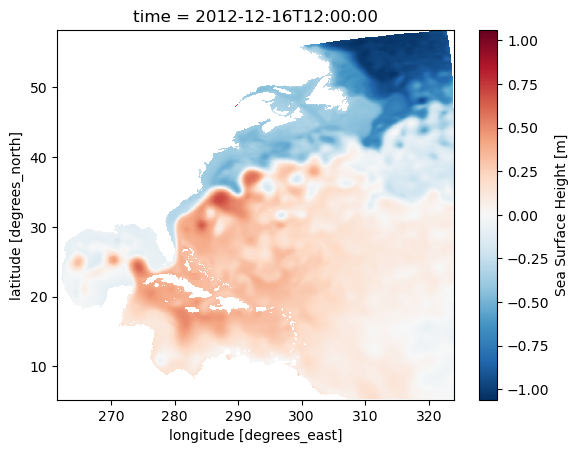
ds.ssh.plot(x='geolon',y='geolat')
<matplotlib.collections.QuadMesh at 0x7f57bbc91a50>