Accessing table (spreadsheet) data

Accessing table (spreadsheet) data#

Packages used#

To use python to access the ERDDAP server directly from your python script or jupyter-notebook, you will need

ERDDAPY
Xarray
netcdf4
matplotlib
folium

Note

The package netcdf4 develop by UNIDATA is not needed in the import part of the python script. However, it is the essential package that support netCDF format output from Xarray. The package matplotlib is also not needed in the import part of the python script. It is the essential package that support quick visualization from Xarray.

In this page, we demonstrate how to extract/download data directly from a ERDDAP server and perform data processing, visualization, and export data in python environment.

Tip

Understanding of the ERDDAP server and what it provides is highly recommended before reading the following intructions.

Import python packages#

import xarray as xr
from erddapy import ERDDAP

xarray is used for data processing and netCDF file output.
erddapy is used to access the ERDDAP server.

Both package-webpages have more detail explanation on its full range of functionalities. Here we will mainly focusing on getting the data to be displayer and downloaded.

Access TableDAP type data#

In this demostration, we will be getting the table data of CPS Trawl Life History Haul Catch Data from NOAA NMFS ERDDAP server

Firstly, the way to use the erddapy is to setup the destination ERDDAP server as an object in python through ERDDAP (a python class)

#### access the ERDDAP server
e = ERDDAP(
    server="https://coastwatch.pfeg.noaa.gov/erddap/",    # The URL that the ERDDAP server has
    protocol="tabledap",                                   # The data type (griddap or tabledap)
    response="opendap",                                   # different output data type that provided by ERDDAP server       
)

Note

Like the comment in the code above, three most important keyword arguments (kwarg) to set for the ERDDAP class are server (The URL that the ERDDAP server is located which has the form of "https://.../erddap/"), protocol (The data type one want to get. It is either "tabledap" or "griddap"), and response (For most general use, set the kwarg as "opendap" to request the data through OPeNDAP Data Access Protocol (DAP) and its projection constraints).

By executing the above code block, we have already setup the connection with the desired ERDDAP server. To request a specific dataset on the server, we need to know the dataset_id. The fastest way to get the dataset ID is to go into the data page (e.g. https://coastwatch.pfeg.noaa.gov/erddap/tabledap/FRDCPSTrawlLHHaulCatch.html). The dataset ID is shown on the second line right after institution.

Tip

One can also get the dataset ID directly from the URL shown above (e.g. https://…/FRDCPSTrawlLHHaulCatch.html).

To set the dataset_id, execute

# set the dataset id name 
#  ex:  https://coastwatch.pfeg.noaa.gov/erddap/griddap/jplAquariusSSS3MonthV5.html
#  dataset_id = jplAquariusSSS3MonthV5
e.dataset_id = "FRDCPSTrawlLHHaulCatch"

Visualize data#

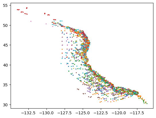
To quickly visualize the different variables (with the help of the installed matplotlib package not imported but supporting the plot method in Xarray),

import numpy as np
cruises = np.unique(ds.cruise.data)

cruises

array([200307, 200403, 200404, 200407, 200503, 200504, 200604, 200704,
       200706, 200804, 200807, 200904, 201004, 201010, 201104, 201204,
       201207, 201208, 201304, 201307, 201404, 201407, 201504, 201507,
       201604, 201607, 201704, 201707, 201807, 201907, 202103, 202107,
       202207, 202307])

import matplotlib.pyplot as plt

for cruise in cruises:
    yy = ds.where(ds.cruise == cruise,drop=True).stop_latitude.data
    xx = ds.where(ds.cruise == cruise,drop=True).stop_longitude.data
    plt.plot(xx,yy,'o',markersize=1)
    

../../../_images/239168809079d8efa0251dee699368bed7688ab3984e96113b8c6572ae614bf7.png

import folium
from folium import plugins

ds.stop_latitude.min().data

lon = (ds.stop_longitude.min().data + ds.stop_longitude.max().data) / 2
lat = (ds.stop_latitude.min().data + ds.stop_latitude.max().data) / 2

fmap = folium.Map(location=[lat, lon], tiles="OpenStreetMap", zoom_start=4)
marker_cluster = plugins.MarkerCluster().add_to(fmap)

for cruise in cruises:
    yy = ds.where(ds.cruise == cruise,drop=True).stop_latitude.data
    xx = ds.where(ds.cruise == cruise,drop=True).stop_longitude.data
    for point in range(0, len(yy)):
        folium.Marker([yy[point],xx[point]], popup=f'Cruise #: {cruise:0.0f}').add_to(marker_cluster)
fmap

Make this Notebook Trusted to load map: File -> Trust Notebook

Preprocess data#

With the help of the Xarray, we can also performed a quick masking on a specific species to see the distribution of the species during the trawling

ds_octo = ds.where(ds.scientific_name=='Octopoda',drop=True)

import folium
from folium import plugins

lon = (ds_octo.stop_longitude.min().data + ds_octo.stop_longitude.max().data) / 2
lat = (ds_octo.stop_latitude.min().data + ds_octo.stop_latitude.max().data) / 2

fmap = folium.Map(location=[lat, lon], tiles="OpenStreetMap", zoom_start=5)
marker_cluster = plugins.MarkerCluster().add_to(fmap)

for cruise in cruises:
    yy = ds_octo.where(ds_octo.cruise == cruise,drop=True).stop_latitude.data
    xx = ds_octo.where(ds_octo.cruise == cruise,drop=True).stop_longitude.data
    for point in range(0, len(yy)):
        folium.Marker([yy[point],xx[point]], popup=f'Cruise #: {cruise:0.0f}').add_to(marker_cluster)
fmap

Make this Notebook Trusted to load map: File -> Trust Notebook

Export to netCDF#

To output the dataset, we use the .to_netcdf() method

ds.to_netcdf('./FRDCPSTrawlLHHaulCatch.nc')

Accessing table (spreadsheet) data

Contents